An illustrated deep-dive into how the compute and comms in TP+SP are overlapped using Async TP
In a previous post we did a deep-dive into Megatron-style tensor parallelism. In this post, we’ll look at an additional optimization building on this prior work: asynchronous tensor parallelism, as described in the paper Overlap Communication with Dependent Computation via Decomposition in Large Deep Learning Models and implemented in PyTorch.
Note other methods1 have been proposed for achieving compute/comms overlap in TP, but this post will focus on the method natively supported in PyTorch, dubbed async TP.
TL;DR
The goal of async TP is to enable full overlapping of the communication and computation that occur in tensor parallelism with sequence parallelism2, to achieve higher device utilization and speed up model training. These all-gather and reduce-scatter comms are typically “exposed” (not overlapped with computation), meaning their latency directly increases training step time and reduces device utilization.
Async TP achieves this overlapping in two ways:
-
Decomposing the blocking, multi-device NCCL collectives into a series of finer-grained async P2P ops executed by copy engines3, dedicated hardware units for direct memory access (DMA) which operates independently of SMs. This prevents any SM contention issues or wave quantization magnification that may occur with SM-based comms kernels.
-
Decomposing the matmuls on each device in the TP group into a series of smaller matmuls, computed in the order the chunks of data arrive via the P2P comms. These submatmuls are executed concurrently with the P2P comms.
In this post we will dive deeper into these concepts and tie them to the actual implementation in PyTorch to make things more concrete. The post is divided into the following sections:
- Background: traditional TP + SP
- Theory
- Translating theory into practice
- Implementation
- Limitations
- Conclusion
Background: tensor parallelism with sequence parallelism
In a previous post I did a deep dive into vanilla tensor paralellism (TP), but a subsequent paper proposed another optimization on top of that: sequence parallelism (SP).
When tensor parallelism is applied to MHA and FFN layers, the ops in between them (dropout, residual, layer norm) are identical, redundant computation on each device, which are cheap to compute but require a lot activation memory. The authors made the observation that these ops are independent along the sequence dimension (e.g., in layer norm we normalize along the feature dimension, it does not cross the batch or sequence dimensions). Therefore, we can actually parallelize the computation across the sequence dimension, while preserving mathematical fidelity with single device training.
This reduces peak activation memory required on each device, and eliminates the redundant computation.
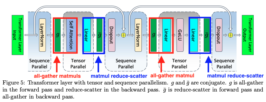
However, there is still one downside to using TP + SP, which is the exposed comms. When transitioning from a SP region to a TP region, we must all-gather the input activations (along the sequence dimension) then perform our usual row-wise/column-wise parallel GEMMs, then reduce-scatter the output activations (along the sequence dimension) to enter the subsequent SP region.
We can see the exposed comms in by looking at a trace of a FFN forward pass in a torchtitan training run with TP+SP. Notice the all-gathers and reduce-scatters are exposed.
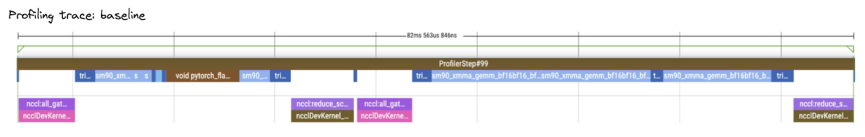
Exposed, blocking comms can result in lower device utilization and increased step time during training. How can we improve this?
Theory
Looped CollectiveEinsum
The authors of the paper Overlap Communication with Dependent Computation via Decomposition in Large Deep Learning Models make 2 observations:
-
An all-gather collective op can be decomposed into a series of async P2P ops that rotate shards of the input activations around the TP group. As soon as a given async P2P op finishes delivering a given shard of the input activation, a submatmul can begin computing a slice of the output immediatley, without waiting for all other shards to be delivered. Conceptually, these output slices are concatenated.
-
A matmul reduce-scatter collective op can be decomposed into a series of async P2P ops that rotate accumulators around the TP group. Each accumulator will be responsible for storing a given shard of the reduce-scattered output. For each iteration, each device computes its portion of the final result that accumulator will hold and adds it the local accumulator. The accumulators rotate round accumulating partial results, and after visiting each device, they contain the full reduce-scattered results.
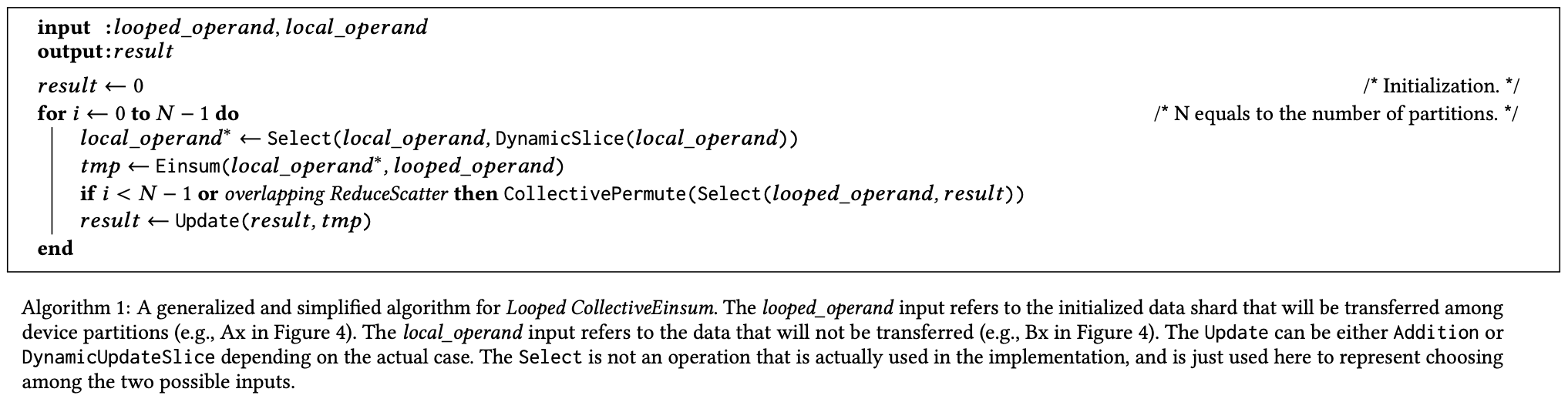
The authors of the paper developed an abstract algorithm called Looped CollectiveEinsum that can generically represent decomposed versions of either all-gather matmuls, or matmul reduce-scatters (see paper snippet above).
However, if you’re like me and this abstract algorithm is not super intuitive in this written form, continue reading below where we’ll break down each decomposition with diagrams for additional clarity.
Note: the paper also covers some additional optimizations in the op scheduling / graph manipulation layer, as well as some kernel optimizations like loop-unrolling, bidirectional data transfer, and more. These won’t be covered in this post, so check out the paper for those details.
Decomposing all-gather matmuls
Let’s walk through this step by step.
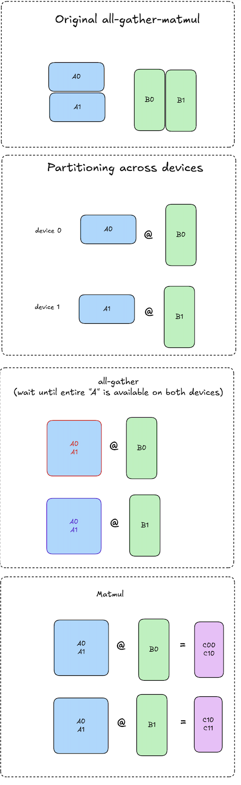
Let \(\textbf{A}\) be the input activations, sharded row-wise:
\[A = \begin{bmatrix} A_0 \\ A_1 \end{bmatrix}, \quad A \in \mathbb{R}^{M \times K}, \quad A_0, A_1 \in \mathbb{R}^{\frac{M}{2} \times K}\]Let \(\textbf{B}\) be the weight matrix, sharded column-wise:
\[B = \begin{bmatrix} B_0, B_1 \end{bmatrix}, \quad B \in \mathbb{R}^{K \times N}, \quad B_0, B_1 \in \mathbb{R}^{K \times \frac{N}{2}}\]In vanilla TP+SP, we all-gather \(\textbf{A}\) on each device, and perform a matmul with the local shard of \(\textbf{B}\) to produce a slice of the output \(\textbf{C}\):
\[C_0 = A \cdot B_0 = \begin{bmatrix} C_{00} \\ C_{10} \end{bmatrix} ,\quad C_1 = A \cdot B_1 = \begin{bmatrix} C_{01} \\ C_{11} \end{bmatrix} \\ \text{where } C_0, C_1 \in \mathbb{R}^{M \times \frac{N}{2}} \text{since B is sharded column-wise}\]Critically, the NCCL all-gather implementation is a blocking, multi-device operation. No device can begin their local matmul until the all-gather has completed on all devices!
The diagrams below visualize this process:
Notation: diagrams use the notation \(A_{i} \cdot B_{j} = C_{ij}\).
The key insight here is that we can actually compute \(A_0 \cdot B_0 = C_{00}\) and \(A_1 \cdot B_0 = C_{10}\) independently, there is no dependency between them.
We can take advantage of this by computing each slice of \(\textbf{C}\) one slice at a time, beginning each computation as soon as we finish pulling a given shard of \(\textbf{A}\) over NVLink, rather than waiting to pull all shards of \(\textbf{A}\).
Furthermore, if we have some mechanism to perform this data movement between devices asynchronously, then we can overlap the pulling of the next shard of \(\textbf{A}\) with the computation using the current shard of A!
The high level algorithm from a single device’s perspective works as follows:
- Let device N begin with input activation shard \(A_N\) present locally on the device.
- Kick off async pull of the shard \(A_{N-1}\) from device N-1.
- Compute \(A_N \cdot B_N = C_{NN}\) locally while async data movement is occurring.
- By the time this matmul is done, the async send/recv op has finished, and we can begin the next matmul immediately: \(A_{N-1} \cdot B_N = C_{N-1,N}\).
- Repeat steps 2-4 until all slices of \(\textbf{C}\) have been computed.
The diagrams below visualize this process:
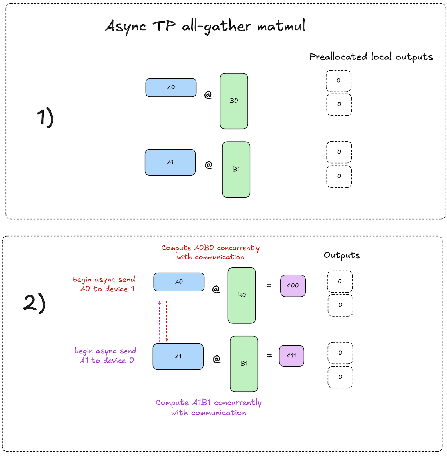
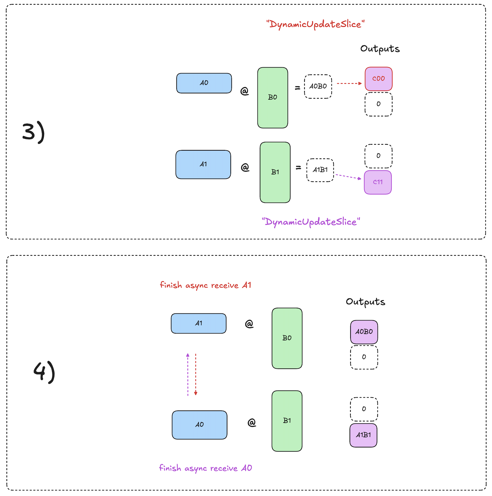
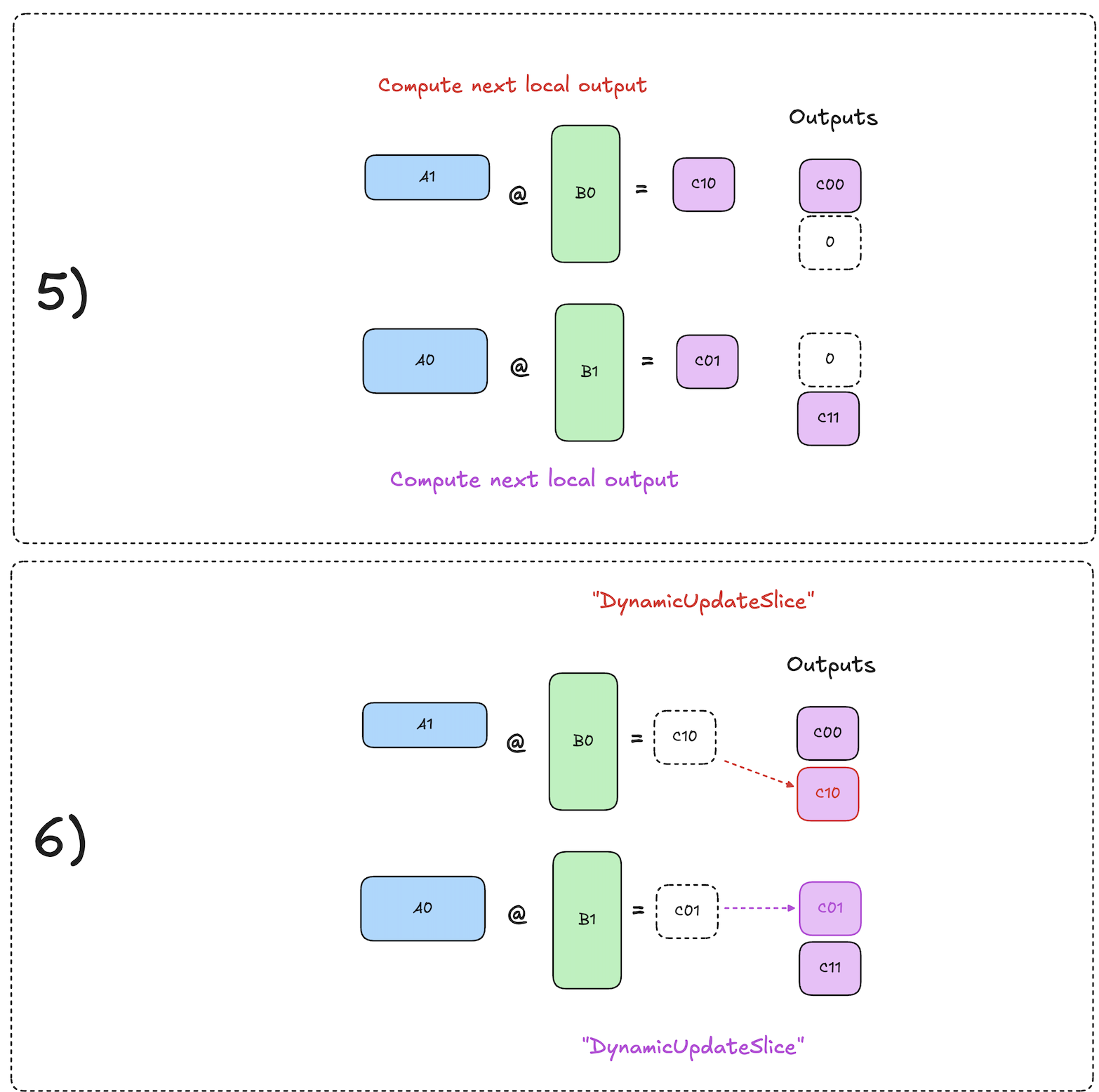
As you can see, the decomposed all-gather has mathematically equivalent results to the original, but with overlapped compute and comms!
Next, we’ll look at how to decompose the matmul reduce-scatter patterns that occur in TP+SP.
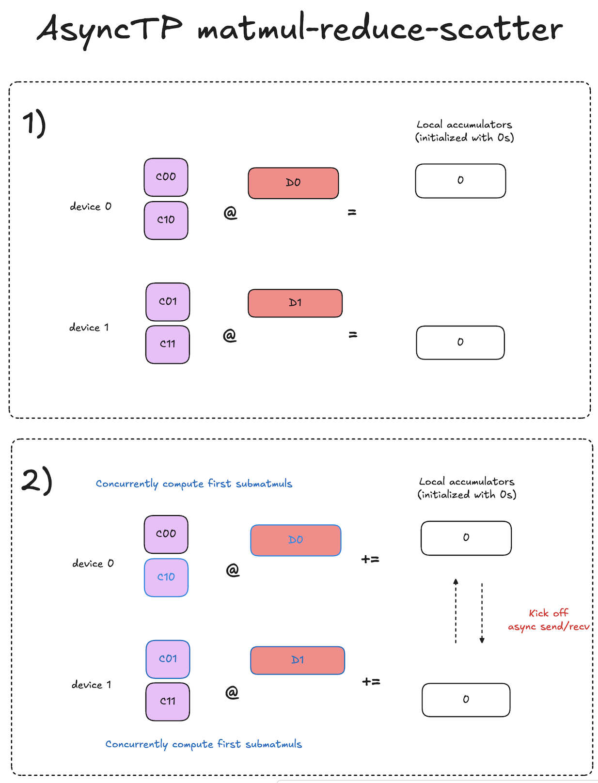
Decomposing matmul reduce-scatters
Decomposing matmul reduce-scatters is a bit tricker to understand, so let’s take it step by step.
The key difference here compared to decomposed all-gather matmuls is that for each iteration we pass around accumulators of partial results, rather than the shards of the input activations. At the end of the process, each accumulator will contain the shard of the final reduce-scattered result that the given local device is responsible for storing.
For each iteration, given a local accumulator that is destined to end up on some other device \(\textbf{D}\) after all iterations are complete, the local device computes its local partial result for that shard of the reduce-scattered result that device \(\textbf{D}\) will store in the end.
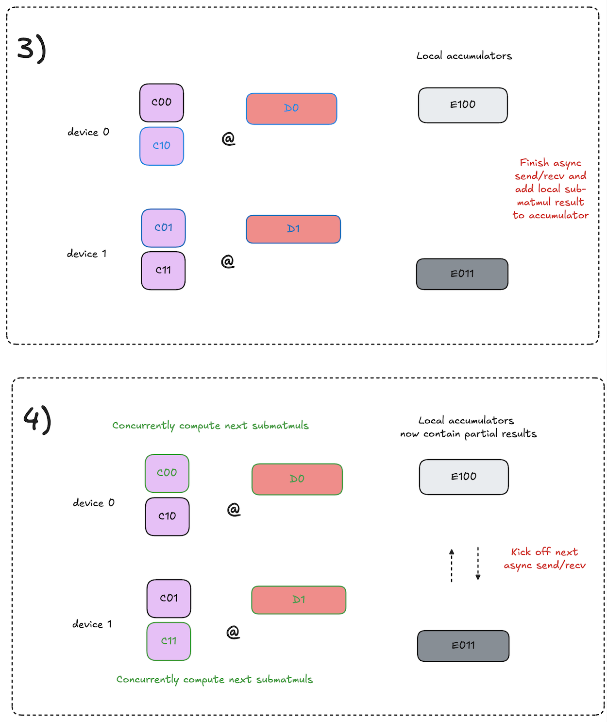
At a high level, the algorithm from a single device perspective works as follows:
- Initialize local accumulators with 0s.
- Kick off async send/recv of accumulators to the next device.
- Concurrently compute the submatmul that will produce partial results for the accumulator that is currently being asynchronously received.
- Add the local partial result to the newly arrived accumulator.
- Repeat steps 2-4 until the accumulators have visited all devices and we have the complete reduce-scattered results on each device.
This process is visualized in the diagrams below. Note that the input activations to the matmul reduce-scatter are the output activations of our prior all-gather matmul.
Notation note: diagrams use notation of \(C_{ij} \cdot D_{k} = E_{ijk}\).
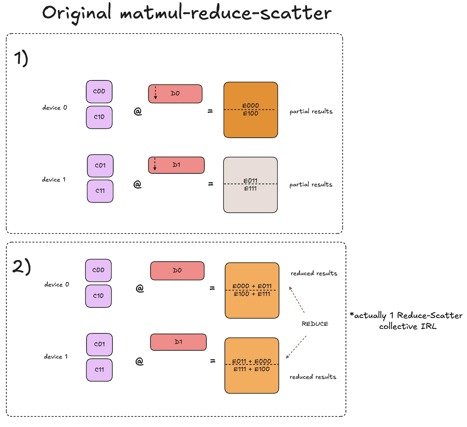
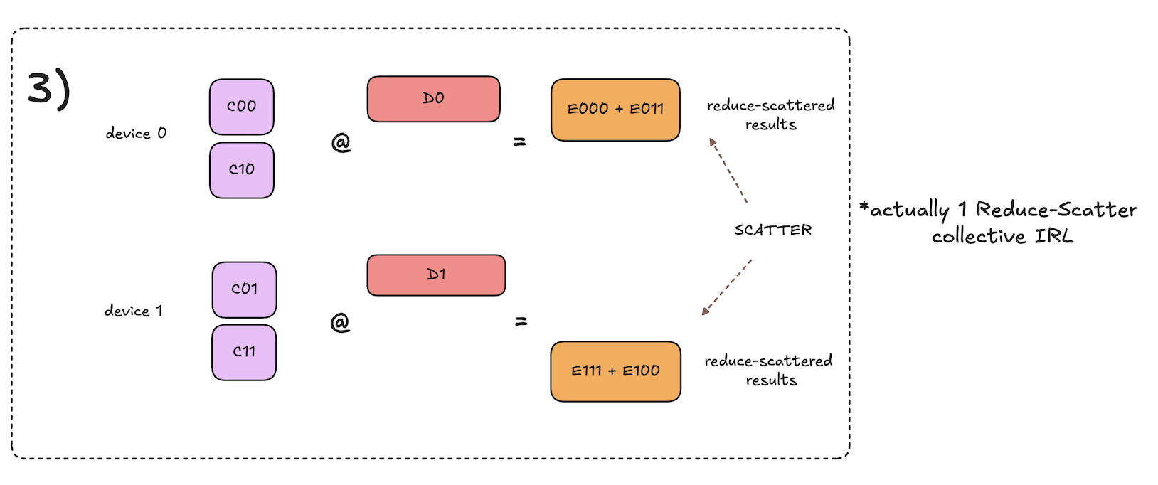
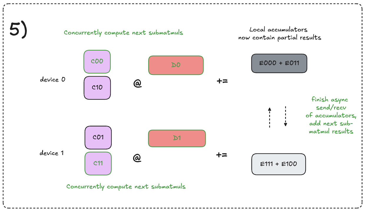
As you can see, the final results of the decomposed matmul reduce-scatter are equivalent to that of the original, but with the communication overlapped with the computation!
Translating theory into practice: challenges at the hardware level
Given this conceptual understanding, we now see that in theory we should be able to overlap the comms and compute for the all-gather matmul.
However, it turns out the implementation details are critical, and a naive implementation can actually yield worse results. Let’s examine why.
Acknowledgement: some of the implementation challenges are outlined in these great posts4 5 on PyTorch’s implementation of async TP, but here I explain it in my own words, providing additional detail and hopefully adding some clarity.
SM contention and wave quantization
Contrary to popular belief, overlapping compute and comms is not an optimization that can necessarily be done “for free” without any trade-offs. The specific hardware units utilized and implementation details matter.
Data movement between GPUs on the same host can be implemented using either SM-based comms kernels or with copy-engines. A naive implementation of the algorithms described above might use common SM-based comms kernels.
However, there are a limited number of SMs on a GPU (e.g., 132 on a NVIDIA H100). This means while these comms kernels running, a reduced number of SMs are available for the concurrent GEMM computation. This amplify the effect of wave quantization, where the number of work units isn’t evenly divisible by the number of available SMs.
Let’s say we have a GEMM with output size (4096,4096) that we divide into tiles of 16x16. This gives us 4096/16 = 256 tiles to compute.
Standard tiled GEMM kernels will try to execute waves of {SM count} tiles, where the individual SMs each work in parallel to compute their assigned tiles. So on a H100 with all 132 SMs available, this will take \(\frac{256 \text{tiles}}{132 \text{SMs}} = 1.94 \text{waves}\).
This means we will do a full wave on 132 SMs, then a partial wave on 124 SMs, to compute the full of 256 tiles. Note that the partial wave takes the same amount of time as the full wave to execute, so this will have the same e2e latency as if it were 2 full waves.
So, what happens if NOT all the SMs are available, due to some being utilized by the NCCL send/recv SM-based comms kernels? Let’s say 6 SMs are being used for comms, leaving 126 SMs for concurrent GEMM computation.
This means our 256 tiles will take \(\frac{256 \text{tiles}}{122 \text{SMs}} = 2.03 \text{waves}\).
We’ll get 2 waves on 122 SMs each, then a 3rd wave on 12 SMs. Remember a partial wave takes just as long as a full wave to execute, so tipping over from 2 waves to 3 wave swill extend the latency of the GEMM operation by ~50%!
Copy-engine based comms
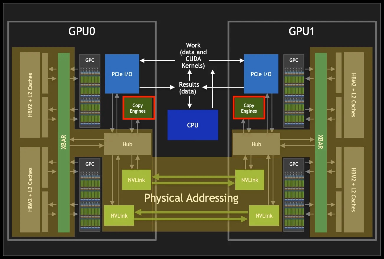
It turns out SMs are not strictly required for all forms of data movement to/from GPU global memory. NVIDIA GPUs have a dedicated hardware unit for direct memory access (DMA) operations. It can perform the following functions:
- Device-to-host (D2H) transfers of data from GPU HBM to CPU RAM.
- Host-to-device (H2D) transfers of data from CPU RAM to GPU HBM.
- Device-to-device transfers of data from one region of GPU HBM to another, on the same device.
- Peer-to-peer (P2P) between GPUs connected via PCIe or NVLink.
By using PyTorch SymmetricMemory APIs, which support P2P ops via copy-engine based kernels, we can avoid the SM contention issue entirely by ensuring the data movement occurs exclusively within these independent, dedicated hardware units. SymmetricMemory APIs basically provide some useful abstractions which take care of the virtual addressing and multicasting operations going on under the hood to facilitate the P2P data access ops.
See the following example, which is from this great post on symmetric memory. I’ve annotated the example to provide additional detail:
import os
import torch.distributed as dist
import torch.distributed._symmetric_memory as symm_mem
import torch

rank = int(os.environ["RANK"])
world_size = int(os.environ["WORLD_SIZE"])
torch.cuda.set_device(f"cuda:{rank}")
dist.init_process_group("nccl")

prev_rank = (rank - 1) % world_size
next_rank = (rank + 1) % world_size

# Allocate a tensor, this will act as our p2p buffer.
t = symm_mem.empty(4096, device="cuda")

# Establish symmetric memory and obtain the handle
hdl = symm_mem.rendezvous(t, dist.group.WORLD)
peer_buf = hdl.get_buffer(next_rank, t.shape, t.dtype)

# Fill p2p buffer `t` with an integer: this device rank.
t.fill_(rank)

# Barrier to ensure all devices have data ready in their p2p buffers.
hdl.barrier(channel=0)

# Allocate a local buffer for the data we're going to pull.
pulled = torch.empty_like(t)

# Move data from peer device p2p buff to local buffer using copy-engine based comms kernel.
pulled.copy_(peer_buf)

# Barrier to ensure all p2p data movement has finished.
hdl.barrier(channel=0)

# Assert that the data in our local buffer has the rank of
# the peer device we pulled from.
assert pulled.eq(next_rank).all()
Great, problem solved! …just kidding - if only it were that easy! We are note quite out of the woods yet.
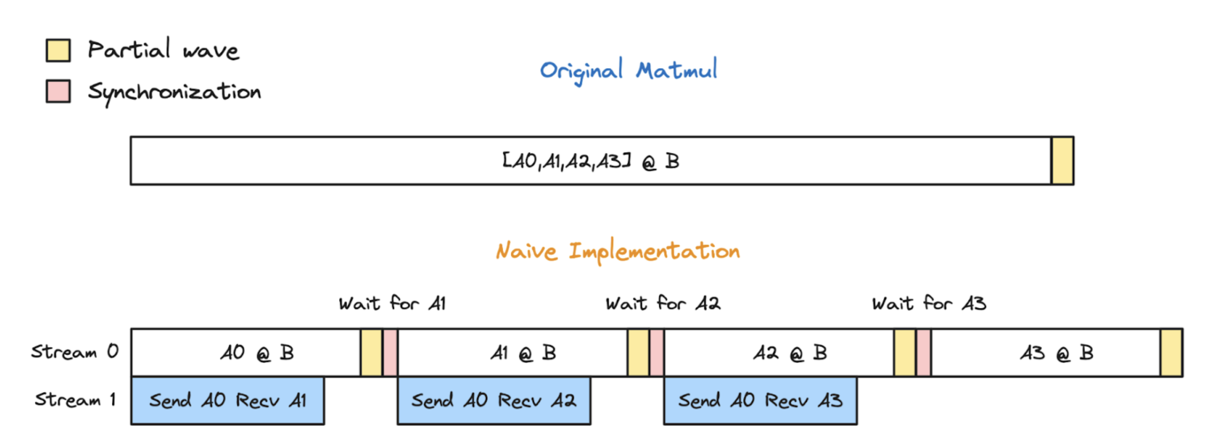
Amplified wave quantization due to decomposition
When using copy-engine based comms, it turns that that depending on other implementation details, we still might find async TP to actually reduce performance. How is this possible?
Well, let’s take the all-gather matmul as an example: in the most common case where the number of tiles is not evenly divisble by the number of SMs available, the original all-gather matmul will require N full waves followed by 1 partial wave, thus we have:
\[\text{Original all-gather matmul waves} = N + 1\]However, if we decompose the all-gather matmul into S (TP group size) submatmuls, depending on the sizes of the submatmuls, we may end up with S waves of size \(\frac{\textbf{N}}{\textbf{S}}\), each of which will have 1 partial wave, thus the total waves required would be:
\[\text{Decomposed all-gather matmul waves} = \left( S \cdot \frac{N}{S} \right) + S \\ \text{Decomposed all-gather matmul waves} = N+S\]As you can see, N+S is greater than N. After all this work, our implementation is still slower!
The following diagram from this great post visualizes this phenomenon:
So, how do we get around this? Well, one way would be to always ensure the total tiles for each decomposed submatmul is evenly divisible by the number of available SMs. However, this is not really feasible, especially in environments where GPUs may be doing other ambient work.
Therefore, PyTorch takes the approach of using two alternating streams. For each iteration, one stream is responsible for executing the compute kernel, and one stream is responsible for executing the copy-engine based comms kernel, and at the end of each iteration, they swap roles.
This allows the next submatmul to begin executing during the partial wave of the previous submatmul, using the remaining SMs not in use by that partial wave. The subsequent submatmul is no longer blocked by the partial wave of the previous one - they can execute concurrently!
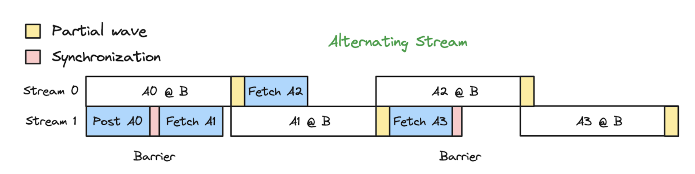
As you can see, this alternating stream approach mitigates the impact of these additional partial waves, since their full latency is not directly impacting the e2e wallclock time. It should be noted that overlapping the partial wave of the previous GEMM “A” with the first wave of the next GEMM “B” can result in some slowdown in the time to finish GEMM B, since it’s first wave is only using the remaining SMs and not the full count of SMs - however, the net result is still an e2e speedup over the original all-gather matmul.
Cool! We’ve discussed a lot of theory and technical details about the nuances of the hardware/software stack - now let’s take a look a little bit of the actual implementation to make things more concrete.
Implementation
Custom ops
Below is the critical section of the PyTorch implementation of a Looped CollectiveEinsum-style decomposed all-gather matmul. I’ve added additional comments and docstrings to walk you through the implementation. This is wrapped with a custom op which makes it traceable for torch.compile.
Note we won’t cover the implementation for the decomposed matmul reduce-scatter here, but if you’re interested here is a code pointer to get you started.
def _pipelined_multi_all_gather_and_consume(
    shard: list[torch.Tensor], # [(shard_dim, K)]
    shard_consumer: Callable[[list[torch.Tensor], int], None],
    ag_out: list[torch.Tensor],# [(shard_dim * group_size, K)]
    group_name: str,
    ag_out_needed: bool = True,
) -> None:
    p2p_workspace_size_req = 0
    for x in shard:
        p2p_workspace_size_req += x.numel() * x.element_size()
    symm_mem = get_symm_mem_workspace(group_name
      min_size=p2p_workspace_size_req,
    )
    group_size = symm_mem.world_size
    rank = symm_mem.rank

    # Start barrier, ensure all members of TP group are ready
    symm_mem.barrier(channel=0)

    # Creates second stream needed for the alternating stream approach.
    backend_stream = _get_backend_stream()

    # New stream waits until current stream finishes queued work and is ready
    backend_stream.wait_stream(torch.cuda.current_stream())

    def copy_shard(dst: list[torch.Tensor], src: list[torch.Tensor]) -> None:
        """
        Async p2p send `s` to `d` to via copy-engine
        by using a simply `copy_` op, which is the API
        provided by symmetric memory.
        """
        for d, s in zip(dst, src):
            d.copy_(s)

    def get_p2p_bufs(remote_rank: int) -> list[torch.Tensor]:
        """
        Get local buffer whose virtual addresses are
        mapped to the physical addresses on the
        `remote_rank` peer device.
        """
        offset_bytes = 0
        bufs = []
        for x in shard:
            buf = symm_mem.get_buffer(
                remote_rank,
                x.shape,
                x.dtype,
                storage_offset=offset_bytes // x.element_size(),
            )
            bufs.append(buf)
            offset_bytes += buf.numel() * buf.element_size()
        return bufs

    local_p2p_bufs = get_p2p_bufs(rank)

    # `ag_out` is an empty output buffer that will
    # contain the all-gathered result after the P2P ops
    # finish running.
    #
    # Here, we are just representing it as lists so
    # the submatmul outputs can be written directly
    # to these sections of the output buffer via indexing
    # like `matmul(a, b, out=shards[i])
    #
    # This correspondds to the diagram in the blog post
    # like so:
    #
    # device 0  [ C00 ] = shards[0][0]
    #           [ C10 ] = shards[0][1]
    #
    # device 1  [ C00 ] = shards[1][0]
    #           [ C01 ] = shards[1][1]
    shards: list[list[torch.Tensor]] = [[] for _ in range(group_size)]
    for x in ag_out:
        for i, y in enumerate(x.chunk(group_size)):
            shards[i].append(y)

    # Parallelization strategy: after each rank copies its shard into its local
    # p2p buffer, every rank issues independent
    # p2p copy -> shard_consumer sequences to two streams.
    # In addition to computation/communication
    # overlapping, the strategy allows
    # for computation/computation overlapping,
    # greatly reducing quantization inefficiency.
    #
    # Notation:
    # - "mv" for the copy to local buffer
    # - "cp" for p2p copies
    # - "b" for barriers
    #
    # Constraints:
    # - The GPU scheduler may or may not overlap "mv"
    # with the first shard_consumer.
    # - "cp" from different streams cannot overlap.
    #
    # Ideal scenario 0 - "mv" overlaps with the first shard_consumer:
    #
    # stream 0: [ shard_consumer ][ cp ][ shard_consumer ]
    # stream 1: [ mv ][b][ cp ][ shard_consumer ]
    #
    # Ideal scenario 1 - "mv" is scheduled before the
    # first shard_consumer:
    #
    # stream 0:       [ shard_consumer ][ cp ][ shard_consumer ]
    # stream 1: [ mv ][b][ cp ][ shard_consumer ]
    #
    # Suboptimal scenario 0 - "mv" is scheduled after
    # the first shard_consumer:
    #
    # stream 0: [ shard_consumer ]               [ cp ][ shard_consumer ]
    # stream 1:                   [ mv ][b][ cp ][ shard_consumer ]
    #
    # Suboptimal scenario 0 - "b" is scheduled after the first shard_consumer:
    #
    # stream 0:       [ shard_consumer ]         [ cp ][ shard_consumer ]
    # stream 1: [ mv ]                  [b][ cp ][ shard_consumer ]
    #
    # We haven't yet figured out a way to ensure "mv" and "b" are either
    # overlapped with or scheduled before the first shard_consumer. Thus, to
    # prevent suboptimal scenarios, we are giving up the chance to overlap "mv"
    # and "b" with the first shard_consumer for now.

    # Copy local shard to p2p buff so other ranks can access it
    copy_shard(dst=local_p2p_bufs, src=shard)

    # Barrier to ensure all ranks have moved data to local p2p buff
    symm_mem.barrier(channel=1)

    # New stream waits on current stream to
    #finish any work and be ready to proceed
    backend_stream.wait_stream(torch.cuda.current_stream())

    # At this point, all ranks have copied their local shard to their
    # local p2p buffer. Each rank can now copy and consume remote shards.
    # Here, we perform the first submatmul with the local shard.
    shard_consumer(shard, rank)

    for step in range(1, group_size):
        # Alternate stream for each rank we iterate through.
        if step % 2 == 0:
            stream = torch.cuda.current_stream()
        else:
            stream = backend_stream

        # For each rank we are pulling data from the remote rank
        # p2p buff to our local shard then doing the matmul.
        remote_rank = (step + rank) % group_size
        remote_p2p_bufs = get_p2p_bufs(remote_rank)
        with stream:
            # Kick off async p2p send/recv via copy-engine.
            copy_shard(
              dst=shards[remote_rank],
              src=remote_p2p_bufs,
            )
            # Execute submatmul.
            shard_consumer(shards[remote_rank], remote_rank)

    if ag_out_needed:
        # Copy from input to the all-gather output. Opportunistically overlap
        # it with the last shard_consumer.
        if group_size % 2 == 0:
            stream = torch.cuda.current_stream()
        else:
            stream = backend_stream
        with stream:
            copy_shard(dst=shards[rank], src=shard)

    torch.cuda.current_stream().wait_stream(backend_stream)
    symm_mem.barrier(channel=0)
Graph manipulation
In the original paper, the authors from Google implement a XLA compiler pass to automatically detect the “all-gather matmul” and “matmul reduce-scatter” ops in the graph of tensor operations, and replace them with the optimized Looped CollectiveEinsum-style implementation.
Likewise, in PyTorch a similar compiler driven approach using pattern matching and graph manipulation is implemented in inductor:
def micro_pipeline_tp_pass(graph: torch.fx.Graph):
    all_gathers = find_all_gather_patterns(graph)
    reduce_scatters = find_reduce_scatter_patterns(graph)

    # When a collective can be hidden through either simple overlapping or
    # micro-pipeline TP, we prefer simple overlapping to avoid the overhead
    # associated with decomposition. If reorder_for_compute_comm_overlap is
    # enabled, we identify collectives that can be hidden through simple
    # overlapping and exclude them from micro-pipeline TP candidates.
    if config.reorder_for_compute_comm_overlap:
        unexposed_collectives = _get_unexposed_collectives(graph)
        all_gathers = [x for x in all_gathers if x.ag_node not in unexposed_collectives]
        reduce_scatters = [
            x
            for x in reduce_scatters
            if x.reduce_scatter_node not in unexposed_collectives
        ]

    if not all_gathers and not reduce_scatters:
        raise AssertionError(
            "async TP found no matching all-gather/reduce-scatter patterns for fusion"
        )

    for all_gather in all_gathers:
        fuse_all_gather_matmul(all_gather)

    for reduce_scatter in reduce_scatters:
        fuse_matmul_reduce_scatter(reduce_scatter)
Here is the code pointer if you wish to trace further into the implementations of the actual graph manipulation. I won’t cover it here since it will be less useful for the average reader, as it uses internal inductor abstractions that would take some time to explain, and frankly, I’m tired after writing this long post :)
Limitations
Some limitations of async TP include:
- NVLink is required.
torch.compileis required, since it uses a compiler driven graph manipulation approach to automatically apply this optimization. So you must be able to compile the model.- The matmuls occuring in the TP regions must be sufficiently large to benefit from this pipelined approach, despite the overhead of decomposition. There is currently no definitive guide/table outlining the expected speedup for different shapes. I will look into adding one.
Conclusion
In this post we walked through the theory and deep technical details of Loop CollectiveEinsum-style decomposed all-gather matmuls and matmul-reduce scatters, as implemented in PyTorch. It was a long journey but we made it! I hope it was as helpful for you to read as it was for me to write.
For an example of how to use async TP in your model, take a look at this code snippet in torchtitan.
Footnotes and references
-
To learn more about the TP+SP parallelization strategy being optimized by async TP, you can read the original paper Reducing Activation Recomputation in Large Language Models or watch my presentatin on the topic here. ↩
-
[Distributed w/ TorchTitan] Introducing Async Tensor Parallelism in PyTorch ↩
-
PyTorch SymmetricMemory: Harnessing NVLink Programmability with Ease ↩