An illustrated deep-dive into Megatron-style tensor parallelism

In this post, I attempt to provide a detailed walkthrough of Megatron-style tensor parallelism, with diagrams to help make the concepts and mathematics more digestible. The target audience for this post is readers who are already familiar with ML and the transformer architecture, who wish to deepen their understanding of tensor parallelism.

The goal of this post is to provide both an overview of the techniques proposed in the paper, as well as a derivation of how we arrive at each particular technique as the best solution, from a set of possible options. We’ll also some examine some of the implementation details of tensor parallelism in PyTorch to make our knowledge more concrete.

This post will be divided into 7 sections, with some broken down into more digestible sub-sections:

1. TL;DR
2. MLP blocks
   • 1st GEMM of the MLP block forward pass - the bad option
   • 1st GEMM of the MLP block forward pass - the good option
   • 2nd GEMM of the MLP block
3. Dropout and layer norm
4. Attention layers
   • Optional attention review
   • Sharding Q,K,V, and O
5. Input embeddings
6. Output embeddings
7. Fusing in the cross-entropy loss

TL;DR

The paper Megatron-LM: Training Multi-Billion Parameter Language Models Using Model Parallelism is a seminal work in ML performance research, and is a must-read for anyone working in this domain. It introduces tensor parallelism as a new technique which

Specifically, TP is applied to:

1. Input embedding
2. MLP blocks
3. Multi-headed self-attention layers
4. Output embedding with fused cross-entropy loss

The computations are carefully partitioned such that:

• The intermediate activations are smaller, reducing peak memory usage and allowing larger models to be trained. Activations often dominate peak memory usage in very large models, so reducing activation memory required to train larger models is important.

• The activations remain sharded for as long as possible before synchronizing (which must be done to ensure the mathematical integrity of the training process), to minimize this communication overhead between devices, which can slow down training and become a bottleneck.

A very high level overview of Megatron-style TP is shown in the diagram below, which is from the paper:

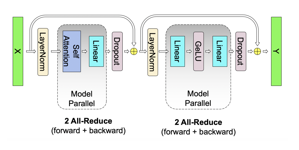
For readers interested in a deep-dive - let’s get started with parallelizing the MLP blocks.

MLP blocks

At the time this paper was written, the standard MLP block following the attention layers in transformers consisted of 2 linear layers with a non-linearity between them ¹. This can be represented mathematically like so:

\[Y = GeLU(XA)\] \[O = YB\]

where X are our input activations, A is the first linear projection, and B is the second linear projection.

Fundamentally, these linear layers will each require 3 GEMM operations.

One in the forward pass:

\[C = AB\]

And two in the backward pass:

\[\frac{\partial L}{\partial A} = \frac{\partial L}{\partial C}B\] \[\frac{\partial L}{\partial B} = \left[\frac{\partial L}{\partial C} \right]^T A\]

The output size of these GEMM operations will be based on the dimensions of the inputs A and the weights B:

\[A \in \mathbb{R}^{M \times K}, \quad B \in \mathbb{R}^{K \times N} \quad \Rightarrow \quad AB \in \mathbb{R}^{M \times N}\]

In the linear projections of the MLP blocks in the GPT-2 style transformer models studied in this paper, M, K, and N are very large (by modern standards they’re actually small, but let’s read the paper in the context it was written in).

Thus, storing all of the intermediate output activations of these GEMMs will be extremely memory intensive. Unless we find a way to reduce this excessive activation memory, we’ll be unable to do research on larger models, due to the current physical limits of HBM capacity on GPUs/TPUs (in this paper, the authors used Tesla V100s with 32GB of HBM).

Thus is born the motivation for the authors to explore reducing activation memory by sharding the matrices involved in these GEMMS across multiple devices. By sharding the computation across devices, each device holds smaller sub-matrices and thus produces smaller activations.

Note: the authors focused on the forward pass when describing the partitioning scheme of the MLP block, so we’ll do the same here, but the same concepts outlined below apply to the backward pass as well.

1st GEMM of the MLP forward pass: the bad option ❌

There are a couple of ways we could shard X and A to reduce the size of output activation. One obvious way is to shard X column-wise and A row-wise. For example, sharding X and A across a tensor parallel group of 2 devices:

\[\mathbf{X} = [X_1, X_2], \quad \mathbf{A} = \begin{bmatrix} A_1 \\ A_2 \end{bmatrix}\]

Conceptually, the math above can be visualized like so (same-colored arrows represent dot products occurring locally on a device):

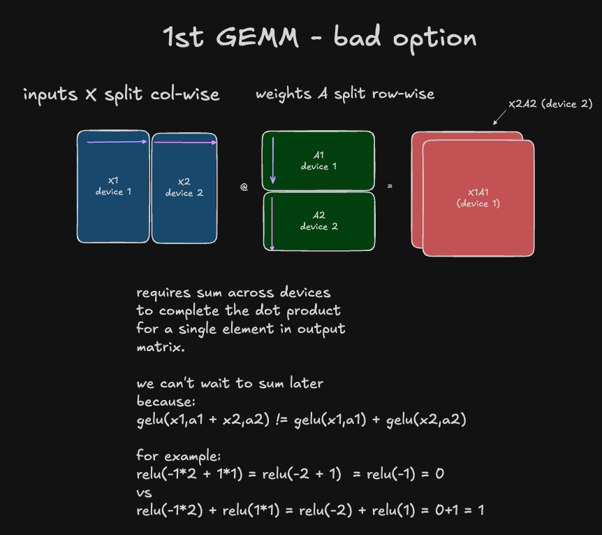
As shown in the diagram above, this option is not ideal because to compute the complete results of any output element in the output matrix, we would need to sum the partial results on each accelerator. This means we already would need an all-reduce operation across all N devices in the tensor parallel group - after only doing the 1st GEMM in the MLP layer! Since we’re trying to minimize the communication overhead by keeping these computations independent on each device for as long as possible, this is probably not ideal, so we should evaluate other options.

However, you might ask: do we necessarily have to all-reduce here? Why can’t we keep the partial results on each device, continue on with applying GeLU to each set of activations individually, do the GEMM for the next linear layer, and then combine these partial outputs via all-reduce at the end?

The answer is because we need this partitioned version of the activation function (left above) to be mathematically equivalent to the original, non-sharded version of the activation function. Otherwise, the integrity of the numerics will be comprised and we’ll run into things like convergence problems, training instability, and so on. In other words: the math will be wrong.

To specific, we can’t perform the GeLU non-linearity on the partial results and sum later because non-linearities like GeLU do not have the distributive property:

\[GeLU(X_1 A_1) + GeLU(X_2 A_2) \ne GeLU(X_1 A_1 + X_2 A_2)\]

Here is an example demonstrating this with a simpler non-linearity (ReLU), and scalar values instead of matrices:

\[\text{ReLU}\left( (-1 \cdot 2) + (1 \cdot 1) \right) = \text{ReLU}(-2 + 1) = \text{ReLU}(-1) = 0\]

vs

\[ReLU(-1 \cdot 2) + ReLU(1 \cdot 1) = ReLU(-2) + ReLU(1) = 0+1 = 1\]

1st GEMM of the MLP forward pass: the good option ✅

So, given that we’d have to perform an all-reduce immediately to maintain mathematical fidelity with the non-sharded computation, let’s examine another option: not sharding the input activations X, and sharding the weight matrix A column-wise:

\[[Y_1, Y_2] = [GeLU(XA_1), GeLU(XA_2)]\]

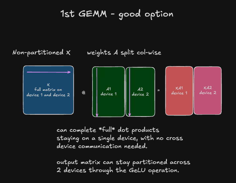
With this approach, there are some immediately obvious benefits:

1) The output activations are still smaller than the original non-sharded version by a factor of \(\frac{1}{\text{number of accelerators}}\) - nice!

2) Since we have complete results for each element of the output matrix on a given device, no summation/reduction operations are necessary and we can apply GeLU directly to these outputs, while maintaining mathematical fidelity with the non-sharded computation - super nice!

With this approach, the activations from the first linear layer now stay partitioned column-wise through the GeLU and pass into the 2nd GEMM.

2nd GEMM of the MLP forward pass

For this final step in the MLP block, there’s no way to avoid synchronization any further:

• Given the activations \(Y\) are sharded column-wise and the activations must be the left operand in the next GEMM \(O = YB\), we can only shard the weights row-wise, so that the number of columns in the left operand (activations) match the number of rows in the right operand (weights) on each device, so we can complete a standard dot product operation. However, the resulting output matrices \([O_1, O_2] = [Y_1 B_1, Y_2 B_2]\) will contain partial results that must be summed across devices before going through the next layer - dropout.

• Matrix multiplication does not have the commutative property (\(AB \ne BA\)). Therefore, we can’t swap around the order of our GEMM operands to make the current column-wise sharding of the activations more favorable, as the mathematics would diverge from the original, non-sharded computation.

Between the two options of sharding the weight matrix \(B\) row-wise or column-wise

The sharded activations flow directly through the 2nd GEMM, where the weights \(B\) of the 2nd linear weight matrix are sharded row-wise across devices.

\[[O_1, O_2] = [Y_1 B_1, Y_2 B_2]\]

Now we have a shard of the complete outputs of the MLP block on each device. We must now (finally) perform an all-reduce to get complete MLP block outputs on each device, in order to go through the dropout layer next.

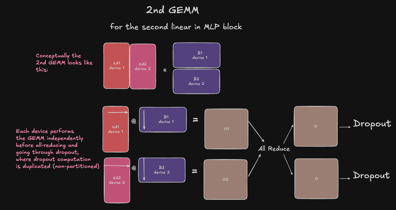
It’s important to remember when we do a collective in the forward pass, we’ll need to perform the inverse of the collective in the backward pass, to propagate the gradient to all relevant inputs, or reduce the gradient from all relevant outputs.

In this case, the all-reduce operation in the forward-pass will become a identity operation (i.e., a no-op) of the upstream gradient across devices.

Conversely, since our input activations to the MLP block were not partitioned in the forward pass (i.e., identity operator), this will become an all-reduce in the backward pass when we need to propagate the gradients from each shard of the computation through to the previous layer. This way our reduced (summed) gradients are exactly equivalent to the gradients of a non-partitioned version of this MLP block.

To recap:

• In the MLP block forward pass, we do only one all-reduce at the end, before the dropout layer. This becomes an identity op in the backward pass.
• In the forward pass, the input activations are not sharded, so this becomes an all-reduce in the backward pass.
• In total, for each MLP block in the transformer, there will be a total of 2 all-reduces: one in the forward pass, and one in the backward pass.

Now that we understand how the MLP block is sharded and why, let’s move on and discuss how dropout and layer norm are handled.

Dropout and layer norm

Now, you may notice that the dropout layer (and layer norm, which is not pictured) are performing redundant computation on every device: after the all-reduce, all devices have the same output activations, and thus applying dropout and layer norm to them will be identical. The authors found simply duplicating this computation is okay because they are relatively computationally cheap, and they did not want to introduce more communication overhead to the model by sharding them.

However, this sets the stage for a future paper, Reducing Activation Recomputation in Large Transformer Models, which observed that layers in the non-tensor parallel regions of the transformer (namely dropout and layer normalization) do not require much computation but do require a lot of activation memory, making them a potentially juicy target for optimization.

They also observed the computation for these layers can be performed independently along the sequence dimension without violating the mathematics - meaning theoretically, they can shard along the sequence dimension and potentially reduce activation memory per device, thus avoiding the need to recompute activations in the backward pass to train larger models. If you’re interested in this, I presented this paper at the Eleuther AI ML Scalability & Performance reading group, which you can check out the recording for here.

Attention layers

Important note: In this paper, the authors explore how to parallelize a vanilla multi-head attention layer. However, it is important to note that the sharding scheme described here is fairly generic and is composable with attention variants such as MQA, GQA, and ring attention, and MLA. There may be slight differences, such as in MQA needing to do redundant projections of \(K\) and \(V\) on each device before applying TP.

So, how do we parallelize the attention layer? It is actually somewhat straight-forward. The reason for this is that MHA has the convenient property that the computation within each attention head is completely self-contained. This makes it easy to parallelize across the num_heads dimension.

Before we go any further, let’s do a brief (optional) review of the matrices involved in the attention layer:

Optional attention review

As a reminder, the multi-head self-attention layer involves the following steps:

1. Our input activations \(X\) are projected through parameter matrices \(W_i^Q\), \(W_i^K\), and \(W_i^V\) to get our queries, keys, and values for each attention head (denoted by the “i” subscript).

\[Q_i = XW_i^Q\] \[K_i = XW_i^K\] \[V_i = XW_i^V\]

Where:

• \(X \in \mathbb{R}^{B \times S \times H}\) are the input activations
• \(W_i^Q \in \mathbb{R}^{d_{\text{hidden}} \times d_q}\) is the query parameter matrix for head \(i\).
• \(W_i^K \in \mathbb{R}^{d_{\text{hidden}} \times d_{kv}}\) is the key parameter matrix for head \(i\).
• \(W_i^V \in \mathbb{R}^{d_{\text{hidden}} \times d_{kv}}\) is the value parameter matrix for head \(i\).
• \(d_q\) is the dimension of queries
• \(d_{kv}\) is the dimension of keys and values
• \(d_{\text{hidden}}\) is the hidden dimension

Our queries, keys, and values are used for scaled dot product attention for each attention head:

\[\text{head}_i(Q, K, V) = \text{softmax}\left(\frac{Q_i K_i^T}{\sqrt{d_{kv}}}\right)V_i\]

Finally, we concatenate our attention head outputs and project them back to the hidden dimension:

\[\text{MultiHead}(\text{head}_1, \ldots, \text{head}_h) = \text{Concat}(\text{head}_1, \ldots, \text{head}_h)W^O\]

Where:

• \(W^O \in \mathbb{R}^{d_{kv} \times d_{\text{hidden}}}\) is the output projection matrix

And now all of our tokens position in embedding space has been updated by aggregating the weighted updates provided by each other token in the context, with weights based on the relevance of each token.

Sharding Q,K,V, and O

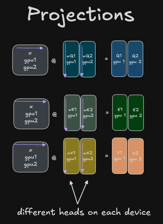
Thus we can shard the \(W^Q\) \(W^K\) \(W^V\) parameter matrices column-wise across the num_heads dimension, as shown in the diagram below. These will operate on our non-sharded input activations which will be coming a previous layer norm layer, which as mentioned previously, is NOT partitioned in any way, so each device has duplicate activations from this layer present on it at this point:

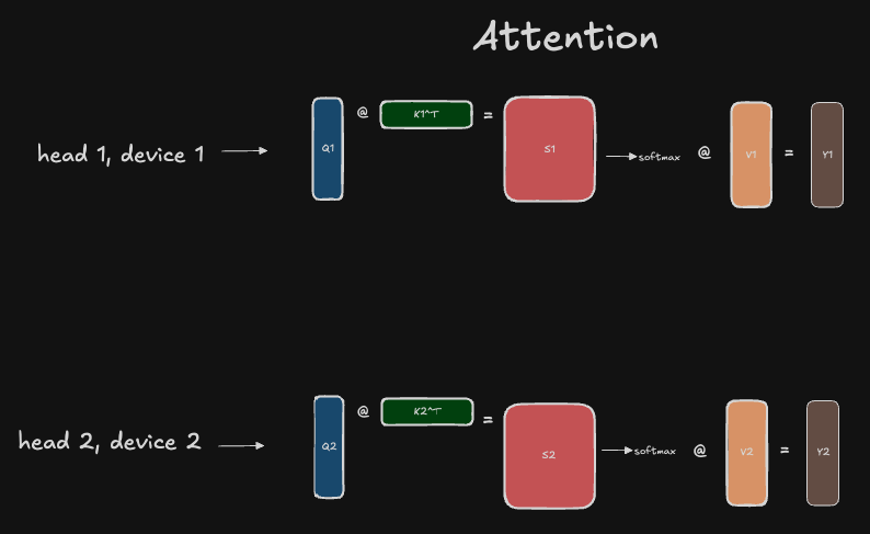
Now that we have our \(Q_i\), \(K_i\), and \(V_i\) projections for each head, we can perform scaled dot product attention for each head locally on each device to get our attention activations for that head, \(Y_i\):

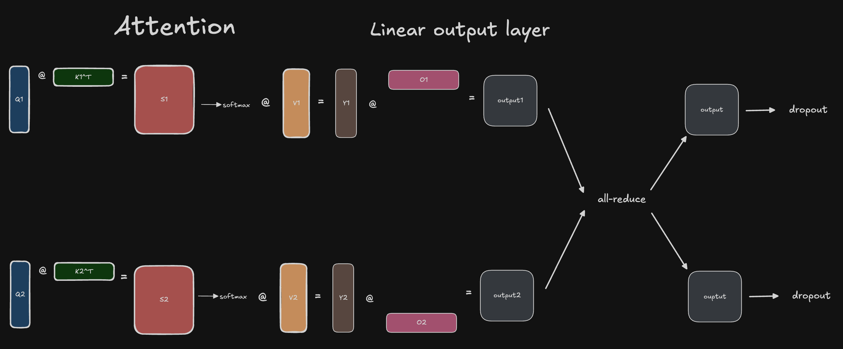
With the attention activations for each head, we can now pass through the final linear projection \(W^O\), which has been partitioned row-wise across devices. As shown in the attention review above, the \(W^O\) projection is normally applied to the concatenated attention heads in the typical unsharded computation. So to maintain mathematical fidelity with the unsharded computation, we now need to all-reduce the outputs before proceeding with the dropout layer:

One natural question may arise at this point: why are we doing an all-reduce here and not an all-gather here? We parallelized along the num_heads dimension, and normally in single-device training we concatenate the attention heads, so wouldn’t the analogous thing to do in multi-device training be to all-gather the head outputs together?

Let’s look carefully at the shapes involved in the computation to figure out why this is.

The local linear projection for each head on each device is:

\[O_i = Y_i W_i^O\]

Where:

• \(Y_i \in \mathbb{R}^{B \times S \times d_{kv}}\) are the attention activations.

• \(W_i^O \in \mathbb{R}^{d_{kv} \times d_{hidden}}\) is the linear output projection.

So the dimensions of the output \(O_i\) will be \(\mathbb{R}^{B \times S \times d_{hidden}}\). Now we can ask ourselves, how would this output shape be different for all the attention heads, instead of just one? Answer: it wouldn’t, none of the dimensions are dependent on the number of heads. So what the output projection is doing is basically performing an aggregated projection using the information in all the attention heads to project the tokens back into the hidden dimension. The diagram below helps illustrate this:

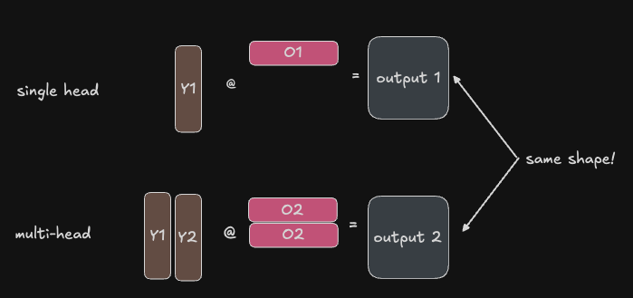
So by parallelizing along the num_heads dimension, we will have the same shaped output activation on multiple devices, each containing only partial results. Therefore, we need to all-reduce to aggregate the results (i.e., the updates to our tokens’ positions in embedding space as dictated by the aggregated updates present in the attention head outputs).

…and that’s it! To recap:

• In the attention layer forward pass, we do only one all-reduce in the forward pass, at the end of the attention layer. This becomes an identity operator (no-op) in the backward pass.
• In the attention layer forward pass, our input activations are not sharded, so this becomes an all-reduce in the backward pass, for the same reasons as described in the MLP section.
• In total, for each attention layer in the model, we’ll have 2 all-reduces: one in the forward pass and one in the backward pass.

Input embeddings

The way the input embeddings are sharded is a bit unintuitive. Let’s start with a diagram then break it down:

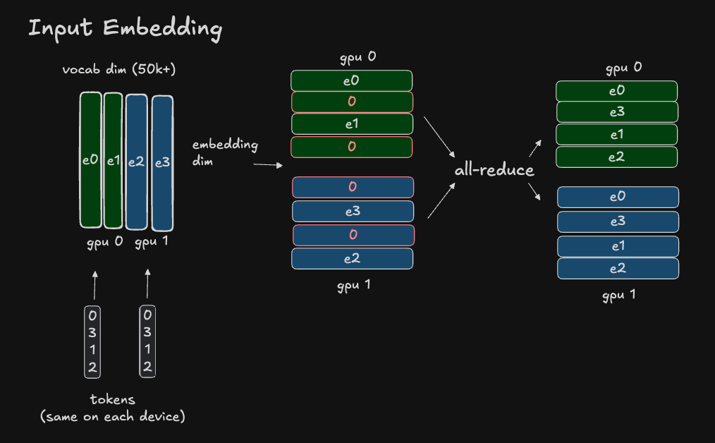
To review, the input embeddings are a matrix \(E_{input} \in \mathbb{R}^{V \times {H}}\) where \(V\) is the vocabulary dimension and \(H\) is the hidden dimension. The embedding matrix basically stores learnable parameters representing the tokens “original” position in embedding space, before any updates to its position (based on the surrounding context) are applied through the various attention layers.

Sharding the input and output embedding matrices is beneficial because the vocabulary size can be quite large (in the paper, it was 50,127 and padded to be 51,200 - the next multiple of 8 - for more efficient GEMMs on the hardware). Since the hidden dimension in this paper is 3072 for the largest model tested (GPT-2 8.2B) the size of the input embedding is:

51,200 tokens * 3072 hidden dimension size = 157,286,400 * 2 bytes per parameter in bfloat16 = 314,572,800 bytes or ~315MB. This can even be much larger in modern models ², so this is good motivation to shard the embedding matrix if possible, to reduce memory pressure and allow other useful things to use that memory.

To shard this embedding matrix, we can do so either row-wise (along the hidden dimension) or column-wise (along the vocabulary dimension).

Sharding along the hidden dimension would require doing an all-gather before going through layer norm (which normalizes along the full hidden dimension). This is not ideal, since all-gather requires moving more data around between devices than all-reduce, which we’ve gotten away with using so far.

For this reason, it turns that by sharding along the vocabulary dimension, we can get away with just using an all-reduce. However, it is a bit unintuitive how this works, so let’s take it step by step.

Sharding along the vocabulary dimension would result in each device having a subset of the token embeddings. At first this seems problematic: our full raw input tokens will arrive on each device in parallel, with shape \(T \in \mathbb{R}^{S \times V}\) where \(S\) is the sequence length and \(V\) is the vocabulary size. How could we handle tokens whose embeddings do not exist on the local device?

We can handle this by simply assigning 0 as the embedding for any token whose embedding does not exist on the device. This scalar 0 can broadcast along the embedding dimension.

So the output of each input embedding on the i-th device is of shape \(Y_i \in \mathbb{R}^{B \times S \times H}\), where some of the tokens along the sequence dimension S have a scalar 0 which broadcasts along the hidden dimension.

Then we can do an all-reduce to get the full token embeddings on each device, with the same shape, but no empty 0 vectors!

To make things more concrete, let’s take a look at the PyTorch implementation of the _MaskPartial Tensor subclass. In particular, let’s look at the _partition_value(...) method:

    def _partition_value(
        self, tensor: torch.Tensor, mesh: DeviceMesh, mesh_dim: int
    ) -> torch.Tensor:
        # override parent logic to perform partial mask for embedding
        num_chunks = mesh.size(mesh_dim)
        # get local shard size and offset on the embedding_dim
        assert self.offset_shape is not None, (
            "offset_shape needs to be set for _MaskPartial"
        )
        local_shard_size, local_offset_on_dim = Shard._local_shard_size_on_dim(
            self.offset_shape[self.offset_dim],
            num_chunks,
            mesh.get_local_rank(mesh_dim),
            return_offset=True,
        )
        # Build the input mask and save it for the current partial placement
        # this is so that the output of embedding op can reuse the same partial
        # placement saved mask to perform mask + reduction
        mask = (tensor < local_offset_on_dim) | (
            tensor >= local_offset_on_dim + local_shard_size
        )
        # mask the input tensor
        masked_tensor = tensor.clone() - local_offset_on_dim
        masked_tensor[mask] = 0
        # materialize the mask buffer to be used for reduction
        self.mask_buffer.materialize_mask(mask)
        return masked_tensor

As you can see, a mask is constructed based on local_offset_on_dim + local_shard_size (basically, the range of indexes that exist on this shard). Any values outside this range are masked and set to 0. The masked ranges on each device are exclusive sets, so every token will have a populated embedding on one device and be set to 0 on all others. When we all-reduce (sum) the resulting token embeddings across devices.

So to recap:

• The input embedding is huge and takes a lot of GPU/TPU HBM capacity to store it, so it’s beneficial to shard it across devices.
• The input embedding is sharded across the vocabulary dimension.
• This requires one all-reduce in the forward pass, which becomes its conjugate (no-op/identity) in the backward pass. Unlike, the MLP and attentions layers, there is no all-reduce in the backward pass. This is because the non-sharded inputs are just the raw token indexes, which we do not compute gradients for, as they are not learnable parameters - so backprop can stop after computing the gradients for the input embedding.

Output embeddings

The output embedding itself is fairly straight-forward, but some complexity arises in how we handle our final cross-entropy loss. Let’s start with a diagram and then break it down:

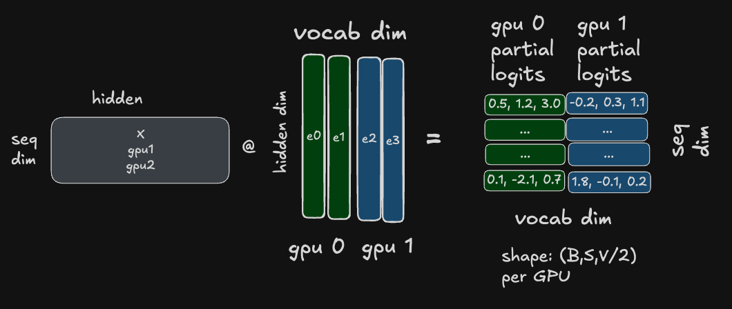
The output embedding is sharded along the vocabulary dimension just like the input dimension. However, in this case, the resulting activation will contain a subset of the logits - the raw scores for each potential next token we can predict at position i in the sequence. We only have a subset of the logits though.

This is the key problem: to compute the softmax probabilities for each sequence, we need access to the full logits (to compute the softmax denominator / normalization factor) - but each device only has a subset of the logits!

So, one natural solution is to perform an all-gather of the logits here, then go through CE loss in parallel. However, this would require sending \(B \times S \times V\) elements between devices.

To reduce the amount of communication overhead here, the authors do something a bit clever, and “fuse” the cross-entropy into this computation. This reduces the amount of data sent over the network to \(B \times S \times N\) where N is the number of devices, and is much, much smaller than V, the vocabulary size ³.

Fusing in the cross-entropy loss

I want to preface this by saying that the authors of the Megatron paper itself provide no details on how they actually fused cross-entropy loss in. Their entire explanation is:

To reduce the communication size, we fuse the output of the parallel GEMM \([Y1, Y2]\) with the cross entropy loss which reduces the dimension to \(b \times s\). Communicating scalar losses instead of logits is a huge reduction in communication that improves the efficiency of our model parallel approach.”

So my understanding of how this works is based on a combination of thinking deeply, diagramming, and reading through the Megatron-LM code base (which has evolved a lot since the original 2021 paper was published). I’ll share what I’ve gathered on how this works below.

Before we dive in, let’s review the cross-entropy loss formula:

\[\text{CE} = -\sum_{i}^{n} p(x_i) log(q(x_i))\]

In this case:

• \(n\) is all the tokens in the vocabulary dimension.
• \(q(x_i)\) is our predicted probability for token \(x_i\)
• \(p(x_i)\) is the true probability of token \(x_i\)

In the case of transformer models, we turn the raw logits for a given position in the sequence i into a probability distribution over the potential output tokens, by using softmax:

\[q(x_i) = \text{softmax}(\text{logits for }x_i)\]

Note that our “true probability” (label) will be 1 for true token, and 0 for all others. Therefore, the CE loss simplifies to:

\[\text{CE} = -\sum_{i=1}^{n} 1 \cdot log(q(x_i))\]

Where:

• \(x_i\) is the “true token” (label)
• \(q(x_i)\) is the models predicted probability for that token.

Now remember the formula for the softmax operation, which we’ll need to compute \(q(x_i)\):

\[\text{softmax} = \frac{e^{q(x_i)}}{\sum_{j=1}^{n}e^{q(x_j)}}\]

Where:

• \(x_i\) is the token in the sequence we are predicting the next token for.
• \(n\) is the range of all possible tokens in the vocabulary.
• \(x_j\) is the current token as we sum over the range of all possible tokens in the vocabulary.

As you can see, the softmax operation requires access to the full range of logits to compute the normalization factor (denominator). However, we only have access to a subset of the logits on each device.

Rather than all-gathering the logits (for the communication overhead reasons described above), we can do the following:

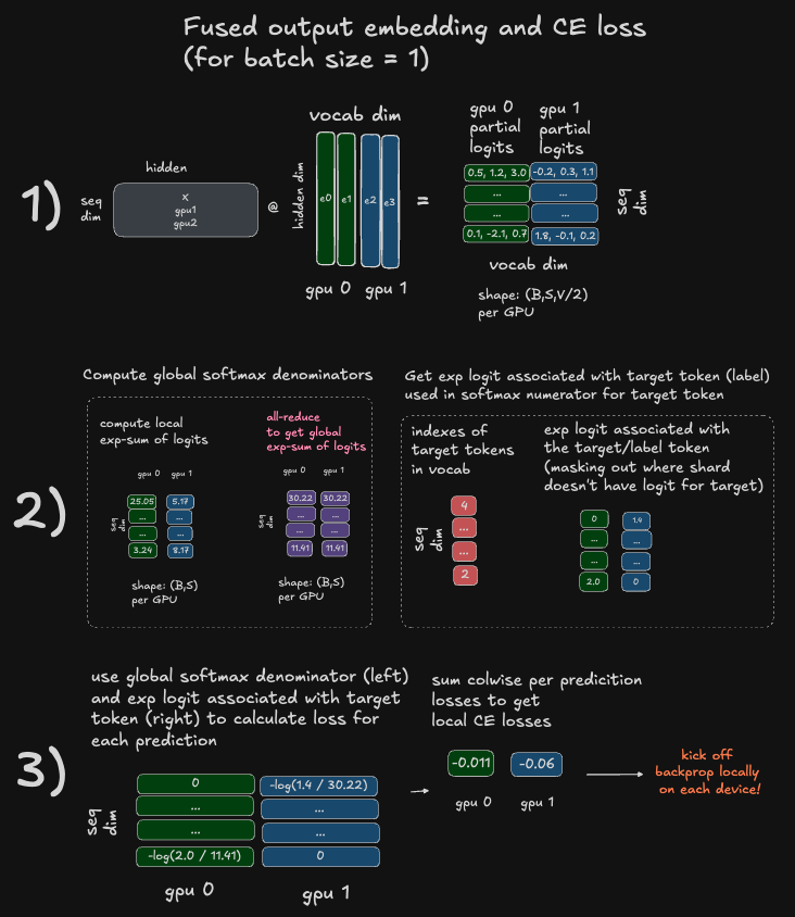
Step 1

• In step 1 of the diagram, we are just computing our logits using the output embedding, as described above. Each device will have a shard of the raw logits.

Step 2

• Starting on the left side of the diagram: compute the local exp-sum \(\sum_{j}^{n}(e^x_j)\) using the local subset of logits available on each device.
  • Now on each device, for each sequence in our batch, we have a single scalar value now representing the local chunk of the softmax normalization factor. This is a total of \(B \times S \times N\) elements, where B is the batch size, S is the sequence length, and N is the number of devices.
• All-reduce to get a global exp-sum (softmax normalization factor). This requires sending the \(B \times S \times N\) elements between devices.
  • Each device now has the the full denominator needed for our loss function.
• For the numerator, we need to compute \(e^{q(x_i)}\) where \(q(x_i)\) is the the model’s predicted probability for the true token (label). Remember though, each local device only has a subset of the logits, so if a true token \(x_i\) is out of the range of our local shard, we set \(q(x_i) = 0\), which is fine because \(e^{0} = 1\).
  • Each device now ha the full global softmax denominator, and the numerators we need for a subset of the predictions.

Step 3

• Starting on the left side of the diagram: compute the local cross-entropy loss. This will only be the partial cross-entropy loss, since each device only computed the loss for the subset of target/label tokens which exist on its local shard of the output embedding.
• Kick off backprop locally! We actually don’t need to do any further reductions to compute the global loss value, since the gradient of the global loss with respect to the local loss would just be 1, since we’re summing them - pretty cool!

Conclusion

Wow, that was a lot. Let’s recap:

• Compared to the full, unsharded model, tensor parallelism reduces the size of the intermediate activation memory needed per device for the tensor parallel regions by a factor of N (number of devices).
• Compared to the full, unsharded model, tensor parallelism adds some communication overhead. Specifically, it adds:
  • 2 all-reduces for each MLP block (one in the forward pass, and one in the backward pass).
  • 2 all-reduces for each attention layer (one in the forward pass, and one in the backward pass).
  • 1 all-reduce for the input-embedding.
  • 1 all-reduce for the output embedding.
  • 1 all-reduce for the fused cross-entropy loss.

Due to this increased communication overhead, the authors limit the size of the tensor parallel group to the Tesla V100s connected via high-bandwidth, low-latency NVLink (8 GPUs, in this case). They studied scaling with pure tensor parallelism, as well as and data parallel + tensor parallel. They found that despite the increased communication overhead, the tensor parallel technique had 76% scaling efficiency up to 512 GPUs. This means that if they achieved N TFLOPs/sec on 1 GPU, with 100% scaling efficiency with 512 GPUs they’d get \(512\cdot N\) TFLOPs/sec, and with 76% scaling efficiency they got \(512 \cdot 0.76 \cdot N\) TFLOPs/sec.

This was pretty good at the time, considering the reduction in peak activation memory allowed them to train models with billions of parameters (which was a lot at the time!).

Closing thoughts

That does it for this post. If you enjoyed it, feel free to join the ML Scalability & Performance research paper reading group I organize, which meets in the Eleuther AI Discord. You can find the Excalidraw diagrams in the post on Github here.

References

• Megatron-LM: Training Multi-Billion Parameter Language Models Using Model Parallelism

Footnotes

1. Nowadays, FFNs with a slightly different structure are often used (see Llama3 models as an example). ↩

2. In more modern transformer models, the hidden dimension can be as high as 16,384 which would require ~1.67GB to store in bfloat16 with the same vocabulary size of 51,200. ↩

3. The authors actually state the amount of elements shared is just \(B \times S\) but after reviewing this several times and discussing with others, I think the \(B \times S \times N\) is the true expression and the authors must have just omitted the N terms since it is relatively small a constant factor (number of devices) that is not dependent on any model dimensions or hyper-parameters. ↩